
Research
Summary
Since October 2021, I am a researcher (Inria Starting Faculty Position) in the MATHERIALS project-team, a joint research team of Inria and École des Ponts ParisTech. My research focus within MATHERIALS is on the development and analysis of sampling methods in high dimensions, in particular for applications related to Bayesian inverse problems and molecular dynamics.
In 2020-2021, I was a postdoctoral researcher at MATHERIALS, working on variance reduction methods for the calculation of transport coefficients in computational statistical physics. Before that, I was a postdoctoral research associate in the group of Applied and Numerical Analysis at Imperial College London. I obtained my PhD in 2019 under the supervision of Prof. Grigorios Pavliotis and Prof. Serafim Kalliadasis. My thesis, which explored several questions in multiscale modeling, is freely available here.
Main research interests
Mean field limit of interacting particle systems
Together with Grigorios Pavliotis and Susana Gomes, we worked on the Desai-Zwanzig mean field model with colored noise. We considered systems of weakly interacting particles driven by colored noise in a bistable potential and we studied the effect of the correlation time of the noise on the bifurcation diagram for the steady-states. More precisely, we considered the following system: \[ \mathrm{d} X_t^i =\left( - V'(X_t^i) - \theta \left(X_t^i - \frac{1}{N} \sum_{j=0}^N X_t^j \right) \right) \, \mathrm{d} t + \sqrt{2\beta^{-1}} \, \xi^i_t \, \mathrm{d} t, \quad 1 \leq i \leq N, \] where \(N\) is the number of particles, \(V(x) = \frac{x^4}{4} - \frac{x^2}{2}\) is the standard double-well potential, \(\theta\) is an interaction strength, \(\beta\) is the inverse temperature of the system, and \(\xi_t^i\) are independent, identically distributed (i.i.d.) noise processes. When these processes are modeled by white noise and the confining potential has multiple minima, particle systems of this type are known to exhibit rich dynamics and, in particular, one or several phase transitions; see (Dawson, 1983), (Tugaut, 2014), and (Gomes & Pavliotis, 2017). Our main aim was to study whether similar phenomena occur in the presence of colored noise, i.e. noise that is not delta-correlated in time. To this end, we developed a spectral method for the nonlinear, nonlocal and nonelliptic Fokker-Planck equation that governs the evolution of the system in the mean-field limit. When the noise is of Ornstein-Uhlenbeck type with characteristic correlation time \(\varepsilon^2\), this equation reads \[ \frac{\partial \rho}{\partial t} = \frac{\partial}{\partial x} \left(V'(x) \rho + \theta \, \left(x - \int_{\mathbb R} x \, \rho(x, \eta, t) \, \mathrm{d} x \right) \, \rho - \sqrt{\beta^{-1}} \, \eta \, \rho \right) + \frac{1}{\varepsilon^2} \frac{\partial}{\partial \eta}\left(\eta \, \rho + \frac{\partial \rho}{\partial \eta} \right). \] A solution of this equation corresponding to a Gaussian initial condition centered at \((1, 1)\) is illustrated below (left), together with the bifurcation diagram for the first moment of the \(x\)-marginal of the solution with respect to the temperature (right).
Figure: Solution of the above McKean-Vlasov equation in the regime where mean-zero solution is stable, in the \((x, \eta)\) plane.
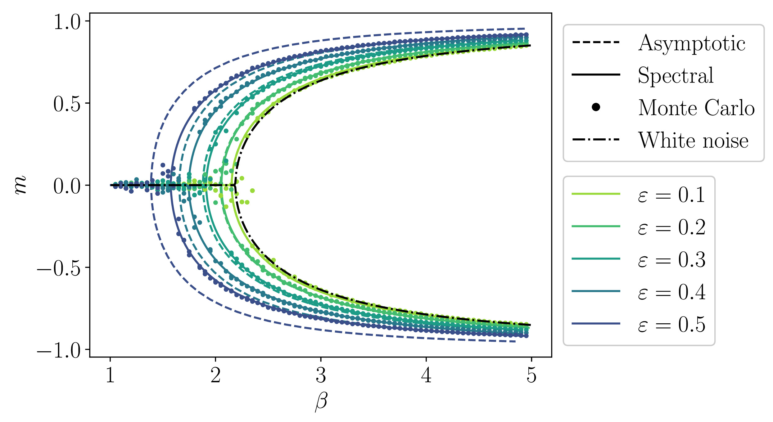
Figure: Approximation of the solution to the Kirchoff-Love plate equation by quadratic discontinuous finite elements, for three different mesh sizes.
This figure in the right panel reveals that the nonzero correlation time of the noise, here parametrized by \(\varepsilon\), leads to an increase of the bifurcation temperature. In general it appeared from our study that, unless the potential in which the noise process is confined is asymmetric, the correlation structure of the noise does not influence the topology of the bifurcation diagram: the mean-zero steady-state solution, which is stable for sufficiently large temperatures, becomes unstable as the temperature decreases below a critical value, at which point two new stable branches emerge, in the same manner as reported in (Dawson, 1983) and (Shiino, 1987). The correlation structure does, however, influence the temperature at which bifurcation occurs, and in general this temperature increases as the correlation time of the noise increases.
- Mean field limits for interacting diffusions with colored Noise: Phase transitions and spectral numerical methods.
- Multiscale Model. Simul.


More recenttly, with José Carrillo, we studied the nonlocal Fokker-Planck equation associated with the ensemble Kalman methodology for inverse problems proposed recently in (Garbuno-Inigo et al., 2019): \begin{align} \frac{\partial \rho}{\partial t}(x, t) = \nabla \cdot \Big( \mathcal C(\rho_t) \left( \nabla \Phi_R(x; y) \, \rho(x, t) + \sigma \nabla \rho(x, t) \right) \Big), \qquad & x \in \mathbb R^d, \, t \in \mathbb R_{\geq 0}, \end{align} where \(\sigma \geq 0\) is a parameter, \(\rho_t = \rho(\cdot, t)\), \(\mathcal C\) is the covariance operator defined by \[ \mathcal C(\rho) = \int_{\mathbb R^d} \left(x - \mathcal M(\rho)\right) \otimes \left(x - \mathcal M(\rho)\right) \, \rho(x) \, \mathrm{d} x, \qquad \text{with } \mathcal M(\rho) = \int_{\mathbb R^d} x \, \rho(x) \, \mathrm{d} x, \] and \(\Phi_R(\cdot; y)\) is a functional of the form \begin{equation} \label{eq:least_squares_functional}% \Phi_R(x; y) = \frac{1}{2} \left|y - \mathcal G(x)\right|_\Gamma^2 + \frac{1}{2} \left|x\right|_{\Gamma_0}^2 =: \Phi(x, y) + \frac{1}{2} |x|_{\Gamma_0}^2. \end{equation} Here \(\mathcal G: \mathbb R^d \rightarrow \mathbb R^{K}\) is a function that, in the terminology of Bayesian inverse problems, is often referred to as the forward model, \(y \in \mathbb R^d\) is a given vector of observations and \(\Gamma \in \mathbb R^{K \times K}, \Gamma_0 \in \mathbb R^{d \times d}\) are symmetric positive definite matrices. We employed the notation \(|\cdot|_{\Gamma} := |\Gamma^{-\frac{1}{2}} \cdot | \), where \(|\cdot|\) is the usual euclidean norm. The covariance-preconditioned Fokker-Planck equation above arises in the mean-field limit of the following interacting particle system, a time discretization of which can be employed to sample from the posterior distribution \(\rho_{\infty} \, \propto \, \mathrm e^{-\Phi_R}\): \[ \dot {X}^{(j)} = - C({\bf X}) \, \nabla \Phi_R(X^{(j)}) + \sqrt{2 C({\bf X})} \, \dot {W}^{(j)}, \qquad j = 1, \dots, J. \] Here \({\bf X} = (X^{(0)}, \dots, X^{(J)})\) is a collection of particles and \(C({\bf X})\) is the associated covariance matrix. In our work, we restricted our attention to the case where \(\mathcal G = G\) is a linear map and we showed that, if \(\rho^1\) and \(\rho^2\) are the solutions of the PDE associated with the initial conditions \(\rho^1_0\) and \(\rho^2_0\), respectively, then a stability estimate of the following form holds: \[ W_2(\rho^1_t, \rho^2_t) \leq C(\rho^1_0, \rho^2_0; G, \Gamma, \Gamma_0) \, \gamma(t) \, W_2(\rho^1_0, \rho^2_0), \] where \(C(\rho^1_0, \rho^2_0; G, \Gamma, \Gamma_0)\) depends only on the first two moments of \(\rho^1_0\) and \(\rho^2_0\) and the function \(\gamma(t)\) converges to zero as \(t \to \infty\) exponentially as \(\mathrm e^{- \sigma t}\) when \(\sigma > 0\) and algebraically when \(\sigma = 0\). This implies in particular the exponential convergence to the equilibrium Gaussian when \(\sigma > 0\), at a rate independent of the initial conditions and of the convexity of \(\Phi_R\), and thereby demonstrates the benefit of the covariance preconditioner for speeding up convergence.
- Wasserstein stability estimates for covariance-preconditioned Fokker-Planck equations.
- Nonlinearity.
The generalized Langevin equation: effective diffusion and long-time behavior
In October 2018, I began to work with Grigorios Pavliotis on the generalized Langevin equation (GLE). In its general form, the GLE is non-Markovian: \[ \ddot q = -V'(q) - \int_{0}^{t} \gamma(t-s) \, \dot q(s) \, \mathrm{d} s + F(t), \] where \(q\) is the position of the particle, \(\gamma\) is a memory kernel, and \(F\) is a mean-zero stationary Gaussian process. The GLE is often used in molecular dynamics and nonequilibrium statistical mechanics to model a particle interacting with a heat bath at equilibrium. Both the dissipation and forcing terms originate from the interaction of the particle with the heat bath; they are related by the fluctuation/dissipation theorem, which stipulates that \[ \mathbb E \left(F(t) F(s)\right) = \beta^{-1} \, \gamma(t-s), \] where \(\beta\) is the inverse temperature; see for example (Pavliotis, 2011). When the memory kernel is of the form \(\langle \mathrm{e}^{-A t} \lambda, \lambda \rangle \), for \(\lambda \in \mathbb R^n\) and \(A \in \mathbb R^{n \times n}\), it is possible to represent the solution as a Markovian process on an extended phase space, making the problem more amenable to analysis: introducing a vector \(z\) of \(n\) auxiliary variables, \((q, p, z)\) satisfy (in law): \begin{align} & \mathrm{d} q = p \, \mathrm{d} t, \\ & \mathrm{d} p = - V'(q) \, \mathrm{d} t + \langle \lambda, z \rangle \, \mathrm{d} t, \\ & \mathrm{d} z = - p \, \lambda \, \mathrm{d} t - A \, z \, \mathrm{d} t + \Sigma \, \mathrm{d} W_t, \qquad z(0) \sim \mathcal N(0, \beta^{-1} I_n), \end{align} where \(W(t)\) is an \(n\)-dimensional standard Brownian motion and the matrix \(\Sigma\) is determined from \(A\) by the fluctuation / dissipation theorem: \(\Sigma \Sigma^T = \beta^{-1} (A + A^T)\). For quasi-Markovian approximations of the GLE, it was proved in (Ottobre & Pavliotis, 2011) that a central limit theorem holds: the rescaled process \(\varepsilon \, q(t/\varepsilon^2)\) converges weakly, in the sense of probability measures on \(C([0, T]; \mathbb R)\), to a pure diffusion: \begin{equation} \label{introduction:central_limit_theorem} \varepsilon \, q(t/\varepsilon^2) \Rightarrow \sqrt{2 \, D} \, W(t), \quad \mbox{in}~C([0, T]; \mathbb R) \quad \mbox{when } \varepsilon \to 0. \end{equation} The coefficient \(D\), which appears as a simple multiplier of the Laplacian in the Fokker-Planck equation associated with the effective diffusion, depends in general on the parameters \(A\) and \(\lambda\) of the quasi-Markovian approximation. This result is illustrated below.
Figure: Illustration of the effective diffusion by Monte-Carlo simulation of the GLE with Ornstein--Uhlenbeck noise; see my thesis for more details on this model of the noise.
Our aim in this project was to study the dependence of the effective diffusion coefficient on the parameters of the equation, and we were particularly interested in three different regimes: the small correlation time, the large friction and the slow friction regimes. To this end we employed formal asymptotics and, in order to verify our results, we developed an efficient numerical method for the hypoelliptic backward and forward Kolmogorov equations associated with the extended Markov process.
We then joined forces with Gabriel Stoltz and obtained rigorous long-time decay estimates, as well as short-time hypoelliptic regularization estimates, for the semigroup associated with the Markov process. From these results, we deduced resolvent estimates that enabled us to prove rigorously (some of) the limits obtained by formal asymptotics.
- Scaling limits for the generalized Langevin equation.
- J. Nonlinear Sci.
Spectral methods for Poisson and Fokker-Planck-Kolmogorov equations
My work on spectral methods for Poisson and Fokker-Planck-Kolmogorov equation, already discussed above in different contexts, began in the first part of my PhD, when I worked with Grigorios Pavliotis and Assyr Abdulle on the investigation, through rigorous analysis and numerical experiments, of a spectral method based on Hermite polynomials for multiscale stochastic equations. More precisely, we developed a numerical method for the solution of multiscale stochastic differential equations (SDEs) of the following type: \begin{align} \mathrm{d} {X}^{\varepsilon}_t = \frac{1}{\varepsilon} f({X}_t^{\varepsilon},{Y}_t^{\varepsilon}) \, \mathrm{d} t + \sqrt 2 \, \sigma_x \,\mathrm{d}{W}_{x}(t), \\ \mathrm{d} {Y}^{\varepsilon}_t = \frac{1}{\varepsilon^2} h({X}_t^{\varepsilon},{Y}_t^{\varepsilon}) \, \mathrm{d} t + \frac{\sqrt 2}{\varepsilon} \sigma_y\,\mathrm{d}{W}_{y}(t), \end{align} where \(X^\varepsilon_t \in \mathbb R^m\), \(Y^\varepsilon_t \in \mathbb R^n\), \(\varepsilon\) is a small parameter encoding the scale separation between the processes \(X^{\varepsilon}\) and \(Y^{\varepsilon}\), \( \sigma_x \in \mathbb R^{m \times m}\), \( \sigma_y \in \mathbb R^{n \times n}\) are constant matrices, and \(W_x\), \(W_y\) are independent \(m\) and \(n\)-dimensional Brownian motions, respectively. When \(\varepsilon \ll 1\), traditional methods for the numerical solution of SDEs are not suitable for this problem, because the time step required to perform a stable and accurate integration in time would be prohibitively small. It is well-known, however, that the slow process \(X^{\varepsilon}\) converges weakly in the limit \(\varepsilon \to 0\) to the solution of a simpler effective equation: \[ \mathrm d X_t = F(X_t) \, \mathrm d t + A(X_t) \, \mathrm d V_t, \qquad X(0) = x_0, \] where \(V_t\) is a standard Brownian motion on \(\mathbb R^m\). The effective coefficients, \(F\) and \(A\), are expressed in terms of the solution to a PDE involving the generator \(\mathcal L_0\) of the fast dynamics, a PDE known as a Poisson equation: \[ -\mathcal L_0 \, \phi(x,y) = f(x,y), \] This equation can be viewed as a PDE on the state-space \(\mathcal Y\) of \(Y^{\varepsilon}_t\) where \(x\) plays the role of a fixed parameter. From the solution to this equation, \(F\) and \(A\) can be obtained as follows: \begin{align} & F(x) = \int_{\mathcal Y} f(x,y) \cdot \nabla_x \phi(x,y) \,\rho^{\infty}(y; x) \, \mathrm d y, \nonumber \\ & A(x) \, A(x)^T = \frac12 \left(A_0(x) + A_0(x)^T\right), \end{align} where \(\rho^{\infty}(y; x)\) is the invariant measure of the fast process for fixed \(X^{\varepsilon} = x\). The convergence (strong, in this simple case) to the solution of the effective equation is illustrated below for the following multiscale system: \begin{alignat*}{2} & \mathrm d X^{\varepsilon}_t = \frac{1}{\varepsilon} X^{\varepsilon}_t \, Y^{\varepsilon}_t \, \mathrm d t, \quad & X^{\varepsilon}_0 = 1, \\ & \mathrm d Y^{\varepsilon}_t = - \frac{1}{\varepsilon^2} \, Y_t^{\varepsilon} \, \mathrm d t + \frac{\sqrt 2}{\varepsilon} \,\mathrm d W_{y}(t), \quad & Y^{\varepsilon}_0 = 0. \end{alignat*}
Figure: Fast \(X^{\varepsilon}\) (top) and slow \(Y^{\varepsilon}\) (bottom) processes for decreasing values of \(\varepsilon\), and comparison with the solution of the effective equation.
For sufficiently small \(\varepsilon\), the slow dynamics can be well-approximated by solving the effective equation instead of the full multiscale system. This approach requires solving the Poisson equation which, when the dimension of the state-space \(\mathcal Y\) is small, can be performed efficiently via a deterministic method. The method we proposed to this end is a spectral method based on Hermite polynomials. Error estimates for the super-algebraic convergence of the method were proved and confirmed numerically with a number of examples, and the method was shown to work extremely well for the simulation of multiscale stochastic partial differential equations.
- Spectral methods for multiscale stochastic differential equations.
- SIAM/ASA J. Uncertain. Quantif.
Finite element methods for elliptic partial differential equations
During my MSc thesis, which I undertook under the supervision of Prof. Jean-François Remacle, I focused on the development of a discontinuous Galerkin method for the Kirchhoff-Love equation, widely used to study the deformation of thin plates subjected to external forces and moments: \[ D \, \Delta^2 w = q, \qquad \mbox{(+ boundary conditions)}. \] Here \(w\) is the vertical displacement, and \(q\) is the load and \(D\) is a rigidity constant. In the first part of the project, the method was implemented and pre-existing theoretical findings were confirmed by means of numerical experiments. In the second part, an analysis was carried out to determine the dispersion and dissipation errors introduced by the numerical scheme, and the method was extended to study buckling phenomena.
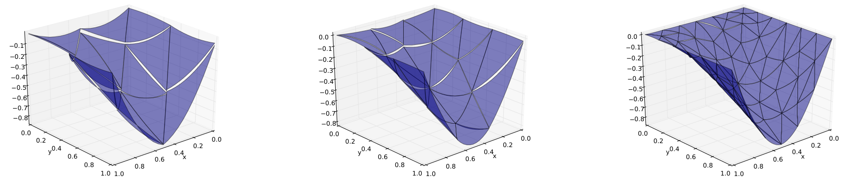
Figure: Approximation of the solution to the Kirchoff-Love plate equation by quadratic discontinuous finite elements, for three different mesh sizes.
- Discontinuous Galerkin method for 4th order elliptic PDEs (in French).
- Unpublished.
My activity in the research area of finite element methods for elliptic PDEs continued in 2016, when I joined the Complex Multiscale Systems group and began to work on the development of a finite element method to solve the Cahn-Hilliard equation with wetting boundary condition: \begin{align} & \frac{\partial \phi}{\partial t} = \Delta \left( \varepsilon^{-1} f_m(\phi) - \varepsilon \Delta \phi \right) \qquad & \mbox{in } \Omega, \\ \\ & \nabla \left( \varepsilon^{-1} f_b(\phi) - \varepsilon \Delta \phi \right) \cdot {\bf n} = 0, \qquad \varepsilon \nabla \phi \cdot {\bf n} = f_w(\phi), \qquad & \mbox{on } \partial \Omega. \end{align} Here \(\phi\) is the phase field, \(f_b(\phi)\) and \(f_w(\phi)\) are functions modeling the bulk and wall energies, respectively, and \(\varepsilon\) is a small parameter encoding the width of the interface. Our aim was to develop a robust method able to tackle engineering problems in multiphase flows. We were particularly interested in modeling the separation of gas-liquid mixtures using a micro-engineering device, an application that we hope to revisit in the future. Examples of numerical results obtained using our method are presented in the figures below.
Figure: Phase field (top) and chemical potential (bottom) during the coalescence of two droplets on a hydropilic substrate.
Figure: Phase field (top) and chemical potential (bottom) for two droplets on hydrophobic substrate.
- A linear, second-order, energy stable, fully adaptive finite-element method for phase-field modelling of wetting phenomena.
- J. Comput. Phys. X.